8.1 Bayesian Networks🔗

Questions around correlation and causation are often asked in the context of complicated probabilistic systems with many variables in it. While probabilistic programs are well-suited for expressing these, it is more common among practitioners to use a more informal language: Bayesian networks. This is a standard language for describing joint distributions over many variables in a structured way. Therefore, we will start by introducing this language. A Bayesian network has two parts: a directed acyclic graph (DAG) and a set of conditional probability tables (CPTs).

A DAG is a network of nodes with edges between them. Each node represents a random variable, and the edges represent a relationship between them (more on what that relationship is later). As the name suggests, the edges have a direction and cannot form a cycle. Here are some common Bayesian network shapes:

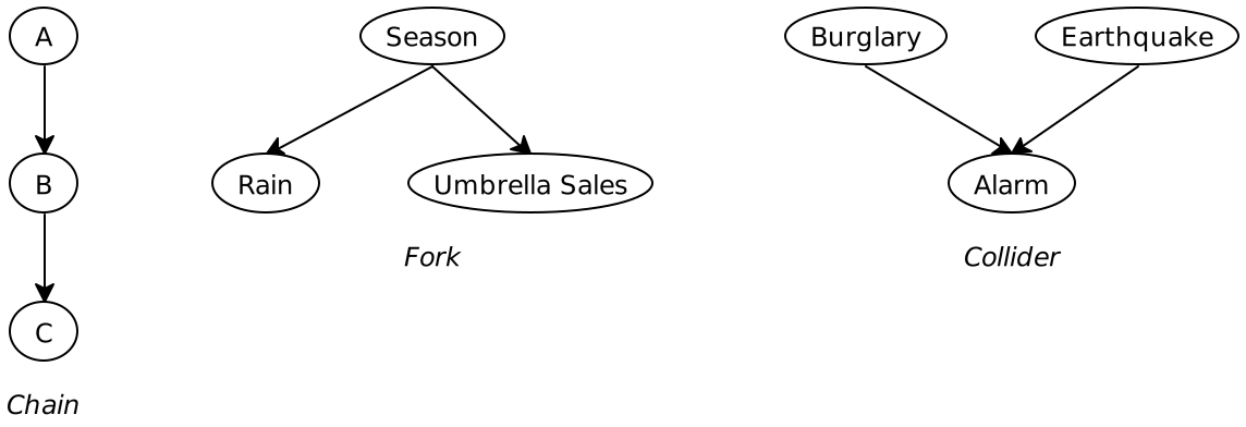
The DAG tells us the qualitative structure of the relationships between the variables, and the conditional probability tables give us a quantification of those relationships. For each node, we have a table with a probability distribution for each possible valuation of its parents. Here is the set of CPTs for the chain example above:

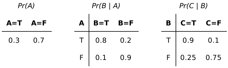
Notice that when a node has no parents, it is just a regular probability distribution. When it does, then it has 2^k distributions, similar to a truth table. As another example, here is the CPT for Pr(Alarm | Burglary, Earthquake) in the collider example:

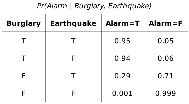
We said earlier that we use Bayesian networks to encode joint probability distributions. How do we get from the data we’ve presented above to a joint distribution? We simply multiply the conditional probabilities implied by the DAG:

\Pr(A = a, B = b, C = c) = \Pr(A = a) \cdot \Pr(B = b \mid A = a) \cdot \Pr(C = c \mid B = b)

There is something important and subtle here: for random variables A, B, C, the above equation does not hold in general. Instead, we have this equation:

\Pr(A = a, B = b, C = c) = \Pr(A = a) \cdot \Pr(B = b \mid A = a) \cdot \Pr(C = c \mid B = b, A = a)

The crucial property that authorizes us to use the first one is the Markov property. Informally, the Markov property is that the probility distribution of a variable is independent from all other variables once its parents are fixed. In this case, it tells us that C ⫫ A \mid B. In general, for a variable Y with parents X_1, ..., X_n, it says that for every other variable Z, we have Y ⫫ Z \mid X_1, ..., X_n.

Try to find how each part of the Roulette program corresponds to the information above.

8.2 Investigating Correlation🔗

So far in this class, all of the probabilistic programs we have written have corresponded to explicitly given relationships between variables. In the real world, however, we often don’t already have access to this information. Instead, we have a soup of measurements, and we have to make sense of them by investigating the relationships between them. The most basic kind of investigation we could do in this situation is to test various possible correlations between the data.

Suppose we have a joint distribution over data we measured in the real world. For example, maybe we have a survey of whether people own a home and own a pet.

> (define (home-and-pet-emp) (make-categorical                           '(((#t #t) . 2/9)                             ((#t #f) . 7/36)                             ((#f #t) . 2/9)                             ((#f #f) . 13/36))))

> (home-and-pet-emp)

┌────────┬───────────┐ │Value   │Probability│ ├────────┼───────────┤ │'(#t #f)│7/36       │ │'(#t #t)│2/9        │ │'(#f #f)│13/36      │ │'(#f #t)│2/9        │ └────────┴───────────┘

We think that these variables might be correlated with one another. Correlation is just another word for "dependence." And we know many ways to check whether two variables are dependent. One way is to check one of their values before and after observing the other.

We can see that the probability of pet is noticeably higher after we observe that someone owns a home. This tells us that there is a correlation between the two. With this information, we are able to write a more structured probabilistic program to encode the same joint distribution:

> (define (home-and-pet-1)       (define home (flip 5/12))       (define pet (if home (flip 8/15) (flip 8/21)))       (list home pet))

> (home-and-pet-1)

┌────────┬───────────┐ │Value   │Probability│ ├────────┼───────────┤ │'(#t #f)│7/36       │ │'(#t #t)│2/9        │ │'(#f #f)│13/36      │ │'(#f #t)│2/9        │ └────────┴───────────┘

We obtain these probabilities by simply querying the original joint distribution: first, we ask it for home to get flip 5/12. Then, we observe! home and query pet to get flip 8/15. If we instead observe! (not home), we get flip 8/21. Putting these together, we get the same joint distribution as before.

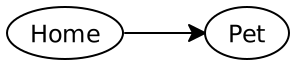
But here’s the problem: probabilistic dependence is symmetric. The program we wrote above essentially exploited this relationship: \Pr(H = h, P = p) = \Pr(H = h) \cdot \Pr(P = p \mid H = h) Corresponding to this Bayesian network structure:

But we equally as well could have reversed the Bayesian network and exploited this relationship instead: \Pr(H = h, P = p) = \Pr(P = p) \cdot \Pr(H = h \mid P = p)

There’s a third option: that both home and pet are derived from a third, unknown common cause. In this context, we often call the common cause a confounding variable. Indeed, the real process for generating the numbers was this:

> (define (home-and-pet-3)       (define high-income (flip 1/3))       (define home (if high-income (flip 3/4) (flip 1/4)))       (define pet (if high-income (flip 2/3) (flip 1/3)))       (list home pet))

> (home-and-pet-3)

┌────────┬───────────┐ │Value   │Probability│ ├────────┼───────────┤ │'(#t #f)│7/36       │ │'(#t #t)│2/9        │ │'(#f #f)│13/36      │ │'(#f #t)│2/9        │ └────────┴───────────┘

This would correspond to a Bayesian network structure like this, where the HighIncome variable was unobserved.

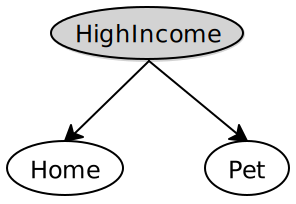
So which of these Bayesian networks is correct? The answer is all three! Bayesian networks, on their own, only express the conditional independence relationship. The data is consistent with all three networks, so we could use any of the three to express the relationship between the variables. Of course, one of these most intuitively corresponds to the actual process in the real world. And this is what brings us to causation.

8.3 Investigating Causation🔗

Of these three networks with are consistent with the data which we have given above, our intuitive "favorite" is like likely the third one. This is because the edges we included in this network correspond to our existing knowledge of the causal relationships between the variables. What do we mean by this? Consider our second Bayesian network:

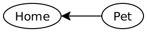
Imagine someone comes along and gifts someone a pet. How does this change the likelihood that this person owns a home? The answer is, of course, not at all. If they owned a home before, they still do, and if they didn’t, they likely still won’t. By contrast, consider the Bayesian network with income included. Suppose someone received a huge raise, and now has a much higher income. This does change the likelihood that they own a home – now that they have more disposable income, they are more likely to be able to take out a loan to purchase one. Similarly, perhaps they are more likely to use their extra disposable income to buy a pet.

A crucial fact to understand about interventions is that they are not equivalent to observations. To illustrate this, let us compare, under this Bayesian network, observing that pet is true and intervening to set it to true.

> (define (home-and-pet-obs)       (define high-income (flip 1/3))       (define home (if high-income (flip 3/4) (flip 1/4)))       (define pet (if high-income (flip 2/3) (flip 1/3)))       (observe! pet)       (list home pet))

> (home-and-pet-obs)

┌────────┬───────────┐ │Value   │Probability│ ├────────┼───────────┤ │'(#t #t)│1/2        │ │'(#f #t)│1/2        │ └────────┴───────────┘

> (define (home-and-pet-itvn)       (define high-income (flip 1/3))       (define home (if high-income (flip 3/4) (flip 1/4)))       (define pet #t)       (list home pet))

> (home-and-pet-itvn)

┌────────┬───────────┐ │Value   │Probability│ ├────────┼───────────┤ │'(#t #t)│5/12       │ │'(#f #t)│7/12       │ └────────┴───────────┘

We have already seen the first operation. When there is a common cause, observing that pet is true increases our likelihood that high-income is true, which in turn increases the likelihood that home is true. The second operation is new. Instead of re-evaluating our likelihood post hoc, we change the data-generating process itself. This leaves the probability of home unchanged, since there is no causal link from pet to home.

So if observational data is insufficient, what do we need? We need experimental data. An experiment is essentially a real-world intervention. Let us consider an example from medicine:

We are considering the effectiveness of Dayquil, a cough medicine which also tends to cause brain fog. We know that Dayquil is correlated with a lower likelihood of having a cough. But perhaps people who take Dayquil are also likely to get rest, perhaps because they take a sick day from work. In order to answer this question, we need to run a controlled experiment. We randomly assign experiment subjects to take Dayquil or not, independent of whether they take a sick day or not.

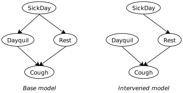
We can then get an estimate of a quantity known as the causal effect, which is the difference in the probability of coughing for someone who takes Dayquil and someone who doesn’t. \big\lvert \Pr(C = T \mid \text{do}\{ D = T\}) - \Pr(C = T \mid \text{do}\{ D = F\}) \big\rvert

When we have experimental data to validate all the relationships in our Bayesian network, we have a causal Bayesian network. This is a Bayesian network which comes with one additional assumption: that the CPTs do not only express the probability distribution of the node if you condition its parents to be a given value, but also the probability if you intervene on its parents to be those values. Interestingly, every Bayesian network we encode in Roulette is already a causal Bayesian network, in the sense that if we change a value, it will affect its children according to the same probability distribution. This is why it is especially important that when we model scenarios with probabilistic programs, we try to do so in a way that makes sense causally.

8.4 Independent Learning🔗

• Encode the Burglary/Earthquake/Alarm example in Roulette. Use the given probabilities the alarm definition. You may make up probabilities for burglary and earthquake

• Compute the causal effect of burglary on alarm. How does this compare to alarm conditioned on burglary? Compute the causal effect of alarm on earthquake. How does this compare the earthquake conditioned on burglary? Why?

• A common source of error in medical experiments is the placebo effect. This is a phenomenon by which a subject who believes themselves to be taking a certain medication shows positive outcomes, even where the medication has no true medical effect. Design a Bayesian network which models the effect of a medication on the presence of a disease, taking into account the placebo effect. What experiment(s) would we need to perform to determine that the actual chemical process of the medication has a causal effect on disease outcome?

References🔗