1 Introduction
| #lang racket | package: base |
The central thesis of this course is that there is a pressing need to make it easier to reason about probabilistic uncertainty and that probabilistic programming languages are a key technology for enabling this. My main aim is to equip you for our modern world, where increasingly we are using computers to automate or augment human decision-making and play a role in our daily lives.
My aim in this course is to:
Equip you to think rationally about complex systems. The world is a complex place, and in order to approach it rationally we require computational abstractions. Probability is a powerful abstraction that has stood the test of time. By the end of this course, you will be able to identify when probability is a useful choice of abstraction, and be familiar with standard probabilistic abstractions that can be used to describe your problem.
Enable you to solve problems with probabilistic components. This is, at its core, a course on problem solving: I want to give you new tools with which you can approach the important problems that occupy every day. These tools will come with mathematical rigor, firm logical foundations, and forms of automation that enable them to scale to practical problems of interest. By the end of this course, you will be able to translate problems in a domain of your choosing into formal probabilistic language in order to deploy a modeling language to solve it.
Familiarize you with the principles of probabilistic modeling languages. A central theme of this course will be modeling languages: languages that are used for describing the world. We will learn their syntax and semantics, and by the end of the course you will be able to select an appropriate modeling language for your problem and know how to design your own modeling language.
Familiarize you with the technical foundations of probabilistic reasoning. How can we teach computers how to reason rationally under uncertainty? This is a question of algorithms and we will approach it as such: we will learn the core algorithmic ideas of probabilistic inference and how to apply them in order to learn the fundamental limitations of how far we can scale probabilistic reasoning. By the end of this course, you will know how to design and implement your own probabilistic reasoning algorithms and deploy them in a probabilistic programming language.
1.1 Why probability?
"Probability is not really about numbers. It is about the structure of reasoning."
– Glenn Shafer
A powerful idea is one that changes how you understand almost everything. It suffuses the world around you, and if you are unaware of it, you are sometimes called ignorant. Physics is a powerful idea: it uses mathematics to explain the relationships between physical quantities, letting us predict the motion of planets and run our cell phones. Chemistry is a powerful idea: it tells us how we are made, and lets us transform one kind of material into another. Computing is a powerful idea: it explains how we formally translate intent into discrete actions, enabling us to design vast systems out of logic that powers much of our modern world.
I believe probability to be one of the very most powerful ideas. I believe probability comes from at least four essential places, but there are certainly more:
Abstraction: Probability is a useful tool for computational abstraction: it simplifies computations by packaging by complicated facts about the world into relative frequencies that are easier to work with.
Algorithmic tool: Probability enables us to write programs with certain desirable properties.
Physics: Some facts about the world are inherently probabilistic and there’s no getting around it.
Deduction: Probability is a powerful framework for combining uncertain knowledge across different sources in order to draw principled conclusions.
Let’s explore each of these in more detail.
1.1.1 Probability as abstraction
How does probability help us abstract and reason about a complex world? The idea likely originated in gambling games, so this is a good place to begin building our intuition. A good example is a simple dice rolling game: your friend rolls two six-sided die, and you want to know: how much should I bet that the sum of these two die is greater than 7?
Important definitions will be written in bold.
Outcome | 2 | 3 | 4 | 5 | 6 | 7 | 8 | 9 | 10 | 11 | 12 |
Relative rate | 1/36 | 2/36 | 3/36 | 1/4 | 5/36 | 6/36 | 5/36 | 4/36 | 3/36 | 2/36 | 1/36 |
The way to read this table is: "the outcome 4 is expected to occur 3 out of every 36 trials of adding up to random dice rolls." Using this table, you can compute that the probability that the dice roll is greater than 7 by summing up the probabilities of the entries for which this is the case:
\Pr(\text{sum of dice roll greater than 7}) = 5/36 + 4/36 + 3/36 + 2/36 + 1/36 = 15
Take a look at your weather app. It probably (hah!) looks something like this:
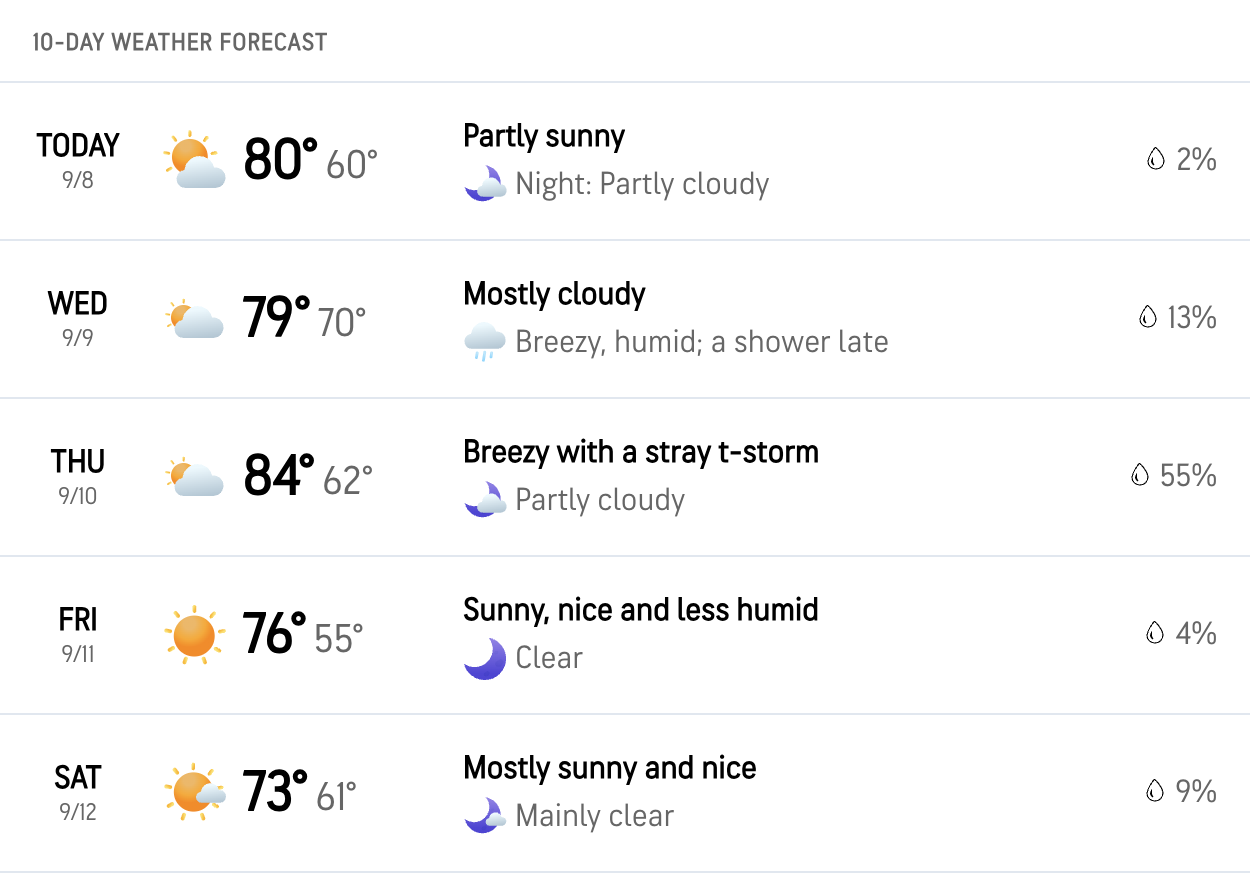
Here your weather app is conveying to you a form of uncertainty: it is saying there is a 2% chance of rain today. You can use this information to choose your wardrobe: probably, you will not wear a rain jacket today. This is an example of probability as a source of abstraction: the physics of the weather and your future movements is too complicated to give you an individual report on what weather to expect in the places you will visit today, so this complexity is summarized as a probability.
1.1.2 Probability as algorithmic tool
Sometimes we want our systems to have some randomness in them. Randomness can play many roles: it can serve as a fair tie breaker, it can encourage the exploration of diverse solutions, it can give provide secrecy and security guarantees, and so on. Avi Wigderson, a Turing award winner, put it this way: "the use of randomness can dramatically enhance computation (and do other wonders) for a variety of problems and settings" (Wigderson 2006).
A prominent example today of randomness providing a tool for designing algorithms is large language models (LLMs). Here, randomness is used a tool to acquire diversity in outputs. Each token it selects is inherently random: in fact, LLMs call random number generators for every token that gets generated, in order to ensure diversity. This is an example of intrinsic randomness intrinsic: it enables the LLM to explore the space of possible productions in a way that provides diversity to the user. But here we see another interesting application of uncertainty: it enables diversity.
The usage of randomness as an algorithmic tool extends far beyond what we might usually consider a computer. Famously, probabilistic uncertainty is everywhere in biology: here it plays many roles, but one prominent role is to encourage diversity in reproduction. Gregor Mendel in his experiments with pea plants showed that genetic traits are inherited according to the laws of probability. Observe the Punnett square, which hopefully you remember from grade school:
Image source: Wikipedia, here
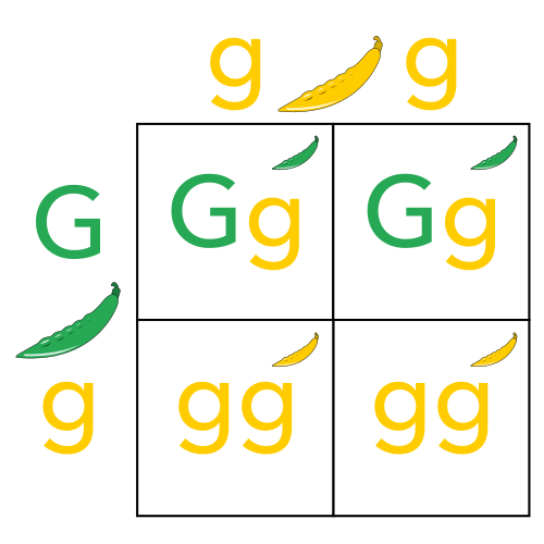
Mendel observed that heritability of certain traits was probabilistic: in the above diagram, we see that breeding one parent with phenotype Gg and the other with phenotypes gg results in 4 possible outcomes for the child phenotype, each with equal probability: Gg, Gg, gg, and gg. Hence, we can conclude that the resulting child is green with probability 1/2, since the dominant trait G is expressed if it is present at all. If one zooms in more on biology, it is probability all the way down. DNA repair and damage is probabilistic, so cancer formation is probabilistic; neuron formation in the brain is probabilistic, and so the process of learning itself is probabilistic; and so on.
Randomness has utility that goes far beyond merely encouraging diversity. Let’s look closely at the Internet and see how it uses randomness. When you type a website into your web browser thousands of random number generators are called. When your computer broadcasts a packet on the network, there is a chance that it conflicts with another computer trying to broadcast at the same time. If this happens, the two computers need to independently decide how to resend their packets without conflicting with each other again. Here it’s randomness to the rescue: the computers choose different random amounts of time to wait to try again, which (with high probability!) de-conflicts them. This is intrinsic randomness: one can show that there is no way to deterministically choose a way to resend packets without conflicts. After your computer talks to the router, one of the first thing it does to secure that connection is generate a "nonce", a special random number that is used as part of a cryptographic handshake between your computer and the router. And so on: each layer of the Internet – from your computer to the router, and then between routers, ultimately all the way to the packet’s destination – is chock full of randomness.
1.1.3 Probability as physical law
Formally speaking, in quantum mechanics, one cannot simultaneously be certain of both a particle’s position and its momentum.
1.1.4 Probability as means of deduction
"In solving a problem of this sort, the grand thing is to be able to reason backwards. That is a very useful accomplishment, and a very easy one, but people do not practise it much."
Spoken by Sherlock Holmes in A Study in Scarlet by Sir Arthur Conan Doyle
Consider the doctor trying to diagnose a patient. How does this interaction proceed?
The doctor comes into the room and the patient complains of some symptoms: a cough, a fever. The doctor asks some questions: where have you been lately? Have you traveled? The patient answers yes: they have been to a few countries. Each of these pieces of information provides a piece of a puzzle, but also has uncertainty: a cough could be a symptom of the disease, or it could be allergies. The patient could be lying. The task of diagnosing the patient is a classic one in probabilistic reasoning: the doctor seeks the most likely disease given observations of the symptoms, which requires smoothly integrating together uncertain information across a huge variety of sources. To solve this problem, today the doctor likely uses his or her brain. But, the question itself can be made a formal mathematical one, which we will seek to formalize and provide tools for in this course.
In this setting, probability can be used as a "faithful guardian of common sense" (Pearl 2014): it can be used to structure internal reasoning and arguments in a way that conforms with our expectations. Probability provides rigor to intuition, and can guide a diagnosis down paths that might not be considered due to bias, distraction, or other human faults.
We will explore the many other motivations for probability as a reasoning tool as we progress through the course, and we will continue to build this list.
1.2 Making it easier to reason about probabilities
The list of places where probability has played a role in our lives goes on and on: if you stare closely at nearly anything in your life, you can find randomness and uncertainty in it. We humans have evolved remarkable capabilities for reasoning rationally about this uncertainty and translating partial information into actions. One goal in this class is to enable a computer to make similar principled decisions about uncertain behavior, and enable it to convey to us its uncertainty to us in a way that we can understand.
My central motivation for this class is this: despite the ubiquity of probabilistic uncertainty in our daily lives and in the sciences, it is still difficult to us to utilize it in our daily lives. We rely on intuitions rather than computations. This has real consequences. Doctors misdiagnose patients; people misunderstand election forecasts and polls; people are scammed by fraudsters and over or underpay for insurance; people lose money gambling; the list goes on and on. My main hope in this class is to make it easier for you – and for other people – to reason about and apply probabilistic arguments in order to reason more rationally about the world.
But for that, we need tools. This class is about those tools.
1.3 Programming in Racket
One of the main themes in this course is that we will use programming languages to understand and reason about probabilistic uncertainty. Do to that, we will need a programming language. We will likely make use of more than one programming language in this course, but for now we start with a nice simple one: Racket. We will begin with Racket because its syntax is very small and its semantics is very easy to explain: we will see how we can describe the majority of the necessary features we will use in Racket in just a few minutes.
You should download and install DrRacket by following the instructions here. If you haven’t used Racket in a while, you should reinstall it to update it. After installing DrRacket and booting it up, it should look like this:
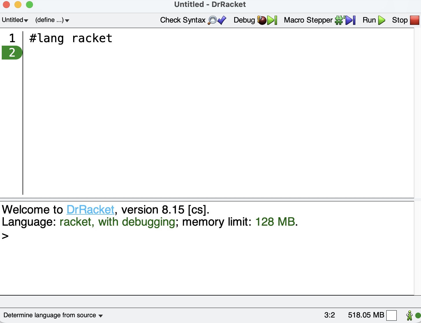
The top pane is called the definition window, and the bottom pane is called the interaction window. The definition window is a text editor you can use to edit a Racket file. The first line this file specifies which programming language you are programming in. In the above example, the first line is:
The interaction window below can be used to interactively execute Racket programs. To load the definitions in the definition window into the interaction window, use the "Run" button in the IDE.
The first concept to understand in Racket is values. Values are programs that do not run to anything. Examples of values include numbers, Booleans, and strings:
> 1 1
> 1/3 1/3
> #t #t
> #f #f
> "hello" "hello"
Comment lines in Racket begin with a semicolon. Everything in Racket is either a value or a function call. Function calls look like this:
> (+ 1 2) 3
The syntax of a function call is (function-name arg1 arg2 ... argn). This calls the + function on the arguments 1 and 2, which runs to the value 3. There are many other functions built into Racket:
> (equal? 1 2) #f
> (* 3 4) 12
> (string-append "hello " "world") "hello world"
Racket’s syntax is uniform and simple. Conditional branching is also a function call:
> (if (> 1 2) "a" "b") "b"
It is common to chain together many if conditionals in a row. Racket provides a convenient built-in function for handling this called cond, which is a multi-way if that executes the first arm that evalutes to #t:
> (cond [#f 10] [#f 30] [#t 20] [#t 50]) 20
Local variables in Racket are declared using the let function:
> (let [(x 10)] x) 10
Note how in the above example we used a square bracket instead of parentheses. In Racket square bracket and parentheses are interchangeable syntax; the choice of which to use is convention and stylistic.
In Racket one defines a function using the lambda keyword, or the λ symbol. Concretely, one can bind a function to a local variable and then call it in the following way:
> (let [(add1 (lambda (x) (+ x 1)))] (add1 10)) 11
1.3.1 Definitions
One can declare named global variables in Racket using the define function, which are typically placed in the definition window:
> (define x 10) > x 10
We can of course define global functions this way as well:
> (define add1 (lambda (x) (+ x 1))) > (add1 10) 11
Here is an interesting function that uses recursion:
> (define (factorial n) (if (equal? n 0) 1 (* n (factorial (- n 1))))) > (factorial 4) 24
1.4 Lists and pattern matching
'(), the empty list value
(cons hd tl), the list constructor that concatenates hd to the list tl
> (cons 1 (cons 2 (cons 3 '()))) '(1 2 3)
Note the syntax '(1 2 3), which is read "quote one two three". This is how Racket renders lists.
It is tedious to type cons all the type so there are a number of short-hand ways to describe lists in Racket:
> (list 1 2 3) '(1 2 3)
There are a number of useful built-in functions for lists; you can see a full list here Here are some examples of some useful ones:
> (define my-list '(1 2 3)) > (empty? my-list) #f
> (length my-list) 3
Now that we’ve built lists, we need a way of destructing them. To do this, we will use the built-in match function:
> (define my-list '(1 2 3))
> (match my-list ['() "empty!"] [(cons hd tl) "not empty!"]) "not empty!"
> (require rackunit)
> (define (sum-list l) (match l ['() 0] [(cons hd tl) (+ hd (sum-list tl))])) > (check-equal? (sum-list '()) 0) > (check-equal? (sum-list '(1 2 3)) 6)
This example also illustrates how to do unit testing in Racket using the rackunit library.
1.5 Structures
A final language feature we will make use of from Racket is structures. For example, here is a binary tree:
> (struct node (l r) #:transparent) > (struct leaf (x) #:transparent)
The #:transparent syntax is boilerplate: it tells the DrRacket REPL that this struct can be printed. Now we can build binary trees:
> (leaf 10) (leaf 10)
> (node (leaf 20) (leaf 30)) (node (leaf 20) (leaf 30))
> (define my-tree (node (leaf 10) (leaf 20)))
> (match my-tree [(leaf n) n] [(node l r) l]) (leaf 10)
Experiment with matching to get a feel for it Here is the detailed documentation for pattern matching if that is helpful. There are many more examples.
1.6 Independent Learning
Some (hopefully most) sessions will end with some independent learning. You should complete these exercises on your own and come ready to discuss them at the beginning of each session.
1.6.1 Reflect on probability
Give three examples of probability in your daily life. Try to be realistic and hunt for it in interesting places. Are there any examples that surprised you? Analyze why the probability is there: is it a means of abstraction, an algorithmic tool, or a means of deduction? Perhaps it is some other reason? If so, identify it.
1.6.2 all-greater?
Implement the function all-greater? l k that takes as input a list of numbers l and number k and returns #t if every element in l is greater than k and #f otherwise. The empty list trivially satisfies the requirement, so (all-greater? '() k) should return #t for any k.
Example:
> (all-greater? '(2 3 4) 2) #f
1.6.3 sum-tree
The following problems use a binary tree datatype whose leaves are numbers:
; type tree = ; | node of tree * tree ; | leaf of number (struct node (l r) #:transparent) (struct leaf (x) #:transparent)
If you’re unfamiliar with structures in Racket, click on the links in the above code to read the documentation. Implement the function sum-tree t that takes a binary tree t as an argument and returns the result of summing all the leaves in the tree.
Example:
> (sum-tree (node (leaf 10) (leaf 20))) 30
Your solution should make use of the match construct.
1.6.4 substitution
Implement a function subst t old n that takes a tree t and two numbers old and n as arguments and returns a tree that results from substituting all leaves of value old with n. This is like a "find and replace" for trees: we want to find all values equal to old and replace them with n, leaving everything else about the tree unchanged.
Example:
> (subst (node (leaf 10) (leaf 20)) 20 30) (node (leaf 10) (leaf 30))