3 Bayesian Reasoning
We are constantly observing facts about the world and updating our state of beliefs about it. We go outside and see that it is cloudy: this increases our confidence that it will rain today. We have a runny nose: we might be getting sick. We are remarkably adept at maintaining a state of belief about how the world works and integrating new information into that state in order to behave rationally.
Your friend rolls 2 dice and tells you their sum.
You bet on the value of the first dice, after hearing their sum.
For example, if your friend tells you that the sum of the two dice is 2, then you can safely bet your life savings on the first dice being 1. But, chances are, your friend won’t give you very good odds on that bet!
Let’s encode this situation into Roulette. First, we roll two dice:
> (define (roll-dice) (make-categorical `((1 . 1/6) (2 . 1/6) (3 . 1/6) (4 . 1/6) (5 . 1/6) (6 . 1/6)))) > (define d1 (roll-dice)) > (define d2 (roll-dice))
Now, suppose your friend tells you the sum of the two dice is 3. We can encode this observation into Roulette using the observe! function:
> (observe! (= (+ d1 d2) 3)) > d1
┌─────┬───────────┐
│Value│Probability│
├─────┼───────────┤
│1 │1/2 │
│2 │1/2 │
└─────┴───────────┘
Now, crucially, the probability of the first dice has changed, because we learned something new. Let’s look at what it is:
> d1
┌─────┬───────────┐
│Value│Probability│
├─────┼───────────┤
│1 │1/2 │
│2 │1/2 │
└─────┴───────────┘
As terminology, we call the probability of d1 before the observation occurs the prior probability of d1, and we call the probability after the observation the posterior probability of d1.
Intuitively, why is this answer correct? We can understand it as follows: the observation restricts the set of events down to those when the observation holds. There are two possible worlds where the event (equal? (+ d1 d2) 3) is #t:
d1=1, d2=2
d1=2, d2=1
Clearly, there are only two possibilities above, and they each have equal probability. So, the posterior probability that d1=1 is 1/2. This process of updating probabilities to incorporate new evidence is called Bayesian updating or Bayesian reasoning. We will see how it is a powerful tool for reasoning about probability distributions and expressing interesting models.
3.1 Medical diagnosis
Suppose you have the following situation: there is a test that can tell you whether or not you have cancer. Before we dive into things, it helps to be very clear about the kinds of outcomes a test like this can have:
A true positive is when they disease is present and the test accurately reports the presence of the disease.
A false positive is when no disease is present but the test inaccurately reports the presence of a disease.
A true negative is when the disease is not present and the test accurately reports the absence of the disease.
A false negative is when the disease is present but the test inaccurately reports the absence of the disease.
The notion of a baseline prevalence is an important simplifying idea in probabilistic modeling. We make an assumption that an average person who walks into the hospital is drawn at random from a uniform pool of all people, who inherently carry some baseline rate of having the disease. This is an example of probabilistic abstraction.
> (define has-cancer (flip 1/20))
> (define test-result (if has-cancer (flip 99/100) (flip 1/5))) > (observe! test-result) > has-cancer
┌─────┬───────────┐
│Value│Probability│
├─────┼───────────┤
│#t │99/479 │
│#f │380/479 │
└─────┴───────────┘
Now we must interpret the above results. We see that, even if the test comes up positive, it is still very likely that this particular patient not in fact have cancer! So, this is not a very informative test.
> (define has-rare-cancer (flip 1/10000000))
> (define test-result (if has-rare-cancer (flip 99999/100000) (flip 1/1000))) > (observe! test-result) > has-rare-cancer
┌─────┬───────────────────┐
│Value│Probability │
├─────┼───────────────────┤
│#t │11111/111122211 │
│#f │111111100/111122211│
└─────┴───────────────────┘
We see that, even though this test seemingly has a very low false-positive rate, it is still overwhelmingly likely that even with a positive test, the person does not have cancer! The moral of this story is: probability is subtle, and humans are often wrong in their intuitions about it.
3.2 Network diagnosis
Work in progress
> (define r1->r2 (flip 0.96))
> (define reaches (if (flip 0.5) (and r1->r2 (flip 0.99)) (and (flip 0.92) (flip 0.98)))) > (observe! (not reaches)) > r1->r2
┌─────┬──────────────────┐
│Value│Probability │
├─────┼──────────────────┤
│#t │0.7031351351351349│
│#f │0.2968648648648651│
└─────┴──────────────────┘
3.3 Bayesian cryptanalysis
Apocryphally, Julius Caesar would tattoo the secret key for his cipher onto the heads of the messengers who delivered his ciphertexts, who would grow their hair before their journey to ensure the key would not be revealed.
The key k is a number between 1 and 26.
To encrypt a letter, shift that letter by k. For instance, encrypting the letter e by the key 2 yields the ciphertext g.
> (define (enc cleartext key) (modulo (+ cleartext key) 26))
> (define (uniform-number low high) (define (make-pairs lo hi num) (if (> lo hi) '() (cons (cons lo num) (make-pairs (add1 lo) hi num)))) (make-categorical (make-pairs low high (/ 1 (- high low))))) > (define key (uniform-number 0 25)) > (enc 1 key)
┌─────┬───────────────────┐
│Value│Probability │
├─────┼───────────────────┤
│16 │0.03999999999999999│
│10 │0.03999999999999999│
│11 │0.03999999999999999│
│12 │0.03999999999999999│
│13 │0.03999999999999999│
│14 │0.03999999999999999│
│15 │0.03999999999999999│
│1 │0.03999999999999999│
│17 │0.03999999999999999│
│2 │0.03999999999999999│
│18 │0.03999999999999999│
│3 │0.03999999999999999│
│19 │0.03999999999999999│
│4 │0.03999999999999999│
│20 │0.03999999999999999│
│5 │0.03999999999999999│
│21 │0.03999999999999999│
│6 │0.03999999999999999│
│22 │0.03999999999999999│
│7 │0.03999999999999999│
│23 │0.03999999999999999│
│8 │0.03999999999999999│
│24 │0.03999999999999999│
│9 │0.03999999999999999│
│25 │0.03999999999999999│
└─────┴───────────────────┘
This looks great! It’s a perfectly uniform output distribution. But, where things get tricky is when we start re-using the same key to encrypt multiple characters. Now, we need a bit of cleverness to see why this is a problem. Suppose we’re an adversary and we see the following ciphertext:
AAFEIACAEAFCAEEFIAJEFF
This text on its own is indecipherable, but we notice something: the distribution of letters we see in the ciphertext is not perfectly uniform. Some letters occur more often than others! For example, it’s well-known that in the English language, the letter "E" is the most common letter: on average, an English letter is "E" about 12% of the time, followed by the letter "T" at 9%, and so on. We can build a large dataset of the English language, and from that we can tabulate the relative frequencies of each letter and summarize them (the power of abstraction!) like this:
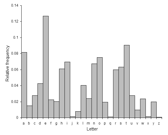
Of course, we can represent this distribution on letters in Roulette:
> (define letter-freqs '((0 . 0.08167) (1 . 0.01492) (2 . 0.02782) (3 . 0.04253) (4 . 0.12702) (5 . 0.02228) (6 . 0.02015) (7 . 0.06094) (8 . 0.06966) (9 . 0.00153) (10 . 0.00772) (11 . 0.04025) (12 . 0.02406) (13 . 0.06749) (14 . 0.07507) (15 . 0.01929) (16 . 0.00095) (17 . 0.05987) (18 . 0.06327) (19 . 0.09056) (20 . 0.02758) (21 . 0.00978) (22 . 0.0236) (23 . 0.0015) (24 . 0.01974) (25 . 0.00074)))
> (define (letter-dist) (make-categorical letter-freqs))
Now we can set up a frequency analysis by observing a particular ciphertext and compute the posterior probability on the key, assuming each letter is drawn from the standard distribution of letter frequencies:
; define cyphertext > (define cyphertext (list 20 17 24 24 1)) ; uniform prior on keys > (define key (uniform-number 0 25)) ; assume each letter drawn from letter distribution > (observe! (equal? (enc (letter-dist) key) 20)) > (observe! (equal? (enc (letter-dist) key) 17)) > (observe! (equal? (enc (letter-dist) key) 24)) > (observe! (equal? (enc (letter-dist) key) 24)) > (observe! (equal? (enc (letter-dist) key) 1)) > key
┌─────┬──────────────────────┐
│Value│Probability │
├─────┼──────────────────────┤
│9 │0.024656516149556593 │
│10 │0.05929006252600924 │
│11 │4.9829784745113537e-5 │
│12 │0.006473545405856663 │
│13 │0.3516355795121869 │
│14 │0.0012875512660878053 │
│15 │1.3039798037913137e-5 │
│0 │0.00358580532673225 │
│16 │0.13825913158756636 │
│1 │5.905071507522831e-6 │
│17 │0.037196339815590625 │
│2 │0.00019043001414818382│
│18 │4.841500589417426e-6 │
│3 │0.0031697178106921743 │
│19 │0.0038040821130813905 │
│4 │2.7325170746876036e-5 │
│20 │0.04499047201637577 │
│5 │0.03355310759807375 │
│21 │0.00024096787650173295│
│6 │0.04418622427022179 │
│22 │0.0012434705647599907 │
│7 │0.019239313652002262 │
│23 │0.0004369335001639928 │
│8 │1.1238044474625339e-6 │
│24 │0.2264586838643183 │
└─────┴──────────────────────┘
We see that the most likely key by far is 13. It turns out that the key here is in fact 13: if we rotate these letters by 13, we get back the plaintext "HELLO". Surely, seeing more text would have given us more information: this plaintext is quite short. There are a few observations I want to make about this example:
We are starting to scale up our examples. Maybe you’re starting to notice something else here: this is quite a big and complicated probability distribution! There are a lot of possible random letters, and a fairly sophisticated constraint being placed on them. There’s no way you would want to calculate this by hand.
Seemingly aggressive probabilistic abstractions can nonetheless yield valid conclusions. Our simplifying assumption about English was extremely aggressive: we assumed every letter was drawn uniformly from the baseline frequency of letters, which clearly not how we ourselves speak English! But, nonetheless, as we observe more data, structure emerges from the abstractions like a crystal forming in solution.
3.4 The common cause
Hopefully by now you’re convinced that probability is essential for making rational inferences about the world, and also that probability can be surprisingly tricky and subtle to work with. To grapple with this, let’s dive deeper into the structure of probabilistic reasoning and begin to build important vocabulary, and get some more experience with modeling and reasoning. We’ll do this by examining more abstract scenarios and observing how probabilities change as we observe things about them, in order to give general principles and phenomena names.
One important phenomenon is the common cause: when two observable outcomes both are caused by the same underlying event. A good example of this is when a disease has two possible observable symptoms. For example, a flu might have the symptoms of coughing and having a fever, which we can model:
> (define has-flu (flip 1/50)) > (define has-cough (if has-flu (flip 3/4) (flip 1/30))) > (define has-fever (if has-flu (flip 1/2) (flip 1/50)))
> has-cough
┌─────┬────────────────────┐
│Value│Probability │
├─────┼────────────────────┤
│#t │0.047666666666666656│
│#f │0.9523333333333334 │
└─────┴────────────────────┘
> has-fever
┌─────┬────────────────────┐
│Value│Probability │
├─────┼────────────────────┤
│#t │0.029600000000000005│
│#f │0.9703999999999999 │
└─────┴────────────────────┘
> (observe! has-cough) > has-fever
┌─────┬───────────────────┐
│Value│Probability │
├─────┼───────────────────┤
│#t │0.17104895104895104│
│#f │0.8289510489510489 │
└─────┴───────────────────┘
Why is this the case? Intuitively, it is because learning that someone has a cough increases the probability that they have a flu, which in turn increases the probability that they have a fever.
3.5 Explaining away
> (define burglary (flip 1/10)) > (define earthquake (flip 1/30)) > (define alarm (if (or burglary earthquake) (flip 4/5) (flip 1/100))) > (observe! alarm) > burglary
┌─────┬──────────────────┐
│Value│Probability │
├─────┼──────────────────┤
│#t │0.709849157054126 │
│#f │0.2901508429458739│
└─────┴──────────────────┘
> earthquake
┌─────┬───────────────────┐
│Value│Probability │
├─────┼───────────────────┤
│#t │0.23661638568470866│
│#f │0.7633836143152913 │
└─────┴───────────────────┘
> (observe! earthquake) > burglary
┌─────┬───────────────────┐
│Value│Probability │
├─────┼───────────────────┤
│#t │0.09999999999999999│
│#f │0.9 │
└─────┴───────────────────┘
Notice how the probability of burglary went down after observing alarm! This is because we learned about what caused the alarm to go off, which greatly reduced the chances of it being caused by the burglary. This is called explaining away: the knowledge of an earthquake explained away the possible burglary.
3.6 Independent learning
3.6.1 The noisy sensors
You are running a moon base and you have three separate sensors that monitor oxygen levels. There are three possible oxygen levels: nominal, low, and danger. Each sensor has a 5% chance of being broken, meaning it outputs a random oxygen level. On average, the oxygen is nominal 98% of the time, low 1.9% of the time, and danger 0.1% of the time. If the sensor is working (95% chance), then there is a 85% chance the sensor outputs the correct oxygen level and a 15% chance it outputs nominal.
Suppose the sensors output nominal nominal danger. Write a Roulette program that outputs the probability that the oxygen level is dangerous in this situation.
3.6.2 The friends at a table
Suppose there are 5 friends named Alice, Bob, Charlie, Derek, and Evan that want to sit around a table with 5 seats. Alice and Charlie do not want to sit next to each other. Write a Roulette program that calculates the probability that Alice sits next to either Evan or Derek.