5.1 Random variables🔗

A random variable is a function out of the sample space. Continuing with our dice rolling example, we can define a function S that maps each pair of dice rolls to their sums, like:

S(⚀⚀) = 2, \quad S(⚀⚁) = 3, \quad S(⚀⚂) = 4, \cdots

The output of a random variable is called its codomain; for instance, the codomain of S above is the set of numbers 2, 3, \cdots, 12. We often denote random variables with capital letters like X or Y. Then, the probability that a random variable X takes on a particular value x, denoted \Pr(X = x), is defined as the total probability of elements in the sample space that X maps to x, i.e.:

\Pr(X = x) = \sum_{\{\omega \in \Omega \mid X(\omega) = x\}} \Pr(\omega)

For example, \Pr(S = 3) = 2/36, since there are two elements of \Omega whose sum is 3, concretely ⚀⚁ and ⚁⚀.

A random variable is simply a variable in a Roulette program. For example, we can define the sum of two dice rolls as:

> (define d1 (make-categorical '((1 . 1/6) (2 . 1/6) (3 . 1/6) (4 . 1/6) (5 . 1/6) (6 . 1/6))))

> (define d2 (make-categorical '((1 . 1/6) (2 . 1/6) (3 . 1/6) (4 . 1/6) (5 . 1/6) (6 . 1/6))))

> (define S (+ d1 d2))

> S

┌─────┬───────────┐ │Value│Probability│ ├─────┼───────────┤ │2    │1/36       │ │3    │1/18       │ │4    │1/12       │ │5    │1/9        │ │6    │5/36       │ │7    │1/6        │ │8    │5/36       │ │9    │1/9        │ │10   │1/12       │ │11   │1/18       │ │12   │1/36       │ └─────┴───────────┘

That the functions make-categorical are in fact special sequences of calls to flip: \Omega really is just a big collection of Boolean assignments.

Often there is more than 1 random variable defined on the same sample space. For example, in the above program, we could also define a random variable even? that is true if the sum is even:

> (define even? (equal? (modulo S 2) 0))

A joint probability distribution is a probability distribution on the outcomes of multiple random variables. As notation, for two random variables X and Y both defined on the same sample space, the joint distribution is written \Pr(X = x, Y = y) for some elements x and y of the codomains of X and Y respectively. We define this probability distribution as:

\Pr(X = x, Y = y) = \sum_{\{\omega \mid X(\omega) = x, Y(\omega) = y\}} \Pr(\omega)

Given a joint probability distribution \Pr(X = x, Y = y), the marginal probability refers to the distribution on a subset of the variables in the joint distribution. Given a joint distribution on 2 random variables, one can compute the marginal on one of them by summing the other out: this is called marginalization. For instance, the marginal distribution on the random variable X is computed from the joint distribution on X and Y as:

\Pr(X = x) = \sum_{y} \Pr(X = x, Y = y)

5.2 Conditioning and Bayes’s rule🔗

We have been working with conditioning in prior lectures via the observe! function, and now we are ready to define its meaning mathematically. Given a joint probability distribution \Pr(X = x, Y = y), the conditional probability of X=x given Y=y is defined as:

\Pr(X = x \mid Y = y) = \frac{\Pr(X = x, Y = y)}{\Pr(Y = y)}

The notation \Pr(X = x \mid Y = y) is read "the probability that X equals x given Y equals y". It helps to visualize the sample space to get a sense for how these quantities relate:

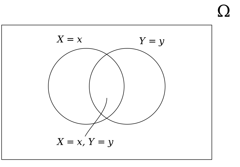
Here we’ve drawn the whole sample space \Omega, and annotated the events where X = x, Y = y, and their intersection. Then, intuitively, we can think of conditioning on Y = y as restricting down to the subset of \Omega where the event Y = y holds. This is why we divide by \Pr(Y = y) in the above: we are renormalizing this restricted probability distribution.

There are a number of useful relationships between the quantities we’ve defined so far. The first is the law of total probability, which combines marginal probabilities with the definition of conditional probability:

\Pr(X = x) = \sum_{y} \Pr(X = x \mid Y = y) \times \Pr(Y = y)

Finally, we have the famous Bayes’s rule, which tells us how to invert conditional probabilities:

\Pr(X = x \mid Y = y) = \frac{\Pr(Y = y \mid X = x) \times \Pr(X = x)}{\Pr(Y = y)}

In the above equation, we call \Pr(Y = y \mid X = x) the likelihood, \Pr(X = x \mid Y = y) the posterior, and \Pr(X = x) the prior, and \Pr(Y = y) is the normalizer. There is nothing particularly fancy about Bayes’s rule mathematically: it simply combines the law of total probability with the definition of conditional probability.

We can compute all these quantities from Roulette programs, and it’s a good exercise to do this. Let’s go back to the medical diagnosis example again, and compute each of these quantities one at a time.

> (define has-cancer (flip 1/20))

> (define test-result (if has-cancer       (flip 99/100)       (flip 1/5)))

In this example, the event Pr(has-cancer = #t) is the prior: we can see by inspecting the program that this is 1/20. The event Pr(has-cancer = #t, test-result = #t) is the likelihood: we can again see by inspecting the program that this is 99/100. The event Pr(test-result = #t) is the normalizer; this is a bit harder to compute by hand, but Roulette makes short work of it:

> test-result

┌─────┬───────────┐ │Value│Probability│ ├─────┼───────────┤ │#t   │479/2000   │ │#f   │1521/2000  │ └─────┴───────────┘

Then, we can compute the posterior manually, and compare it with what we get out of Roulette:

> (/ (* 1/20 99/100) 479/2000)

99/479

> (observe! test-result)

> has-cancer

┌─────┬───────────┐ │Value│Probability│ ├─────┼───────────┤ │#t   │99/479     │ │#f   │380/479    │ └─────┴───────────┘

We see these two numbers agree! So, Roulette is properly using Bayes’s rule to compute posterior probabilities.

5.3 Independence and dependence🔗

Relationships between random variables are one of the central ideas in probability, and one of the simplest and most important kinds of relationships is independence. Let \Pr(X, Y) be a joint probability distribution on random variables X and Y. Then, X and Y are independent random variables if their joint probability is the product of their marginals, i.e. that for any x and y it is the case that:

\Pr(X = x, Y = y) = \Pr(X = x) \times \Pr(Y = y)

If two random variables X and Y are independent, we denote this as X ⫫ Y.

Independence is a very restrictive property: in most interesting probabilistic programs, there are limited examples of independence. What is far more prevalent is conditional independence, which states that two random variables X and Y are rendered independent if you condition on a third random variable Z; this is denoted X ⫫ Y \mid Z. Concretely, X and Y are conditionally independent given Z if we have that for any x,y,z, it holds that:

\Pr(X = x, Y = y \mid Z = z) = \Pr(X = x \mid Z = z) \times \Pr (Y = y \mid Z = z)

Conditional independence is quite prevalent in probabilistic programs: it occurs whenever all influence of one random variable on another flows through a third. For instance, consider the following program:

> (define X (flip 1/3))

> (define Z (if X (flip 1/4) (flip 1/5)))

> (define Y (if Z (flip 1/8) (flip 1/9)))

In this program, we have that X ⫫ Y \mid Z. We can see this using observe!:

> (observe! Z)

> (and X Y)

┌─────┬───────────┐ │Value│Probability│ ├─────┼───────────┤ │#t   │5/104      │ │#f   │99/104     │ └─────┴───────────┘

You should perform the calculations yourself to see that this is in fact evidence of conditional independence.

5.4 A note on references and sources🔗

I have, over the years, gained a collection of opinions on books that introduce probability, which I can summarize here if you are interested in explore more of the formal foundations of probabilistic reasoning:

•  (Jaynes and Bretthorst 2003) is a classic introduction to probability with a compelling introduction that puts probability theory in the context of formal logic and reasoning. There is a good account of decision theory.

•  (Murphy 2022) gives a great introduction to probability in the context of machine learning, and is a very good reference for advanced continuous probabilistic concepts.

•  (Pearl 2014) gives a good account of probability in the context of Bayesian networks, and is particularly useful as a historical point of view on how probability was motivated to the artificial intelligence community in the 1970s, which was very skeptical of probabilistic reasoning and much more inclined towards formal logic (my how times change!)

•  (Graham et al. 1994) has a great chapter on probability, and it heavily inspired the presentation here.

5.5 Independent learning🔗

• Show that, if X and Y are independent random variables, then \Pr(X = x \mid Y = y) = \Pr(X = x) for any x and y.

• Write a Roulette program indep? a b that checks if two Bernoulli random variables are independent or not. Your code will need to use the query function.

References🔗