2 Knowledge Compilers
| #lang racket | package: base |
Last time we discussed in detail how knowledge compilers can play a valuable role in the design and implementation of probabilistic programming languages. In this lecture we will discuss the foundations of knowledge compilation on its own.
2.1 A knowledge compilation map
Knowledge compilation (KC), broadly speaking, is concerned with the study of syntactic representations of logics. The core insight of KC to categorize different syntactic representations by their various properties (Darwiche and Marquis 2002). This is an idea quite familiar to programming-languages-oriented people, but was quite exotic for those steeped in SAT solvers and other propositional reasoning strategies.
Let’s see a simple example: the propositional language Formula. This language has the following surface syntax:
\varphi, \psi ::= x \mid \varphi \lor \psi \mid \varphi \land \psi \mid \neg \varphi \mid T \mid F
And, it has the following abstract syntax:
> (struct Band (l r) #:transparent) > (struct Bor (l r) #:transparent) > (struct Bneg (e) #:transparent) > (struct Bvar (v) #:transparent) > (struct Btrue () #:transparent) > (struct Bfalse () #:transparent)
A propositional language has a semantics in terms of propositional logic. Let’s quickly give this language a semantics. Let \Gamma be a set of logical variables. Then, a formula \varphi is well-formed in context \Gamma, written \Gamma \vdash \varphi, if the following inductive relation holds:
\dfrac{~}{\Gamma \vdash T} \qquad \dfrac{~}{\Gamma \vdash F} \qquad \dfrac{x \in \Gamma}{\Gamma \vdash x} \dfrac{\Gamma \vdash \varphi \quad \Gamma \vdash \psi} {\Gamma \vdash \varphi \land \psi} \qquad \dfrac{\Gamma \vdash \varphi \quad \Gamma \vdash \psi} {\Gamma \vdash \varphi \lor \psi} \qquad \dfrac{\Gamma \vdash \varphi}{\Gamma \vdash \neg \varphi}
Intuitively, this relation simply asserts that every syntactic logical variable in \varphi is contained in \Gamma. Now we can give a semantics to contexts, which simply maps each logical variable in \Gamma to a truth value:
\llbracket \Gamma \rrbracket : \Gamma \rightarrow \{T, F\}
And finally we are ready to give a semantics for Formula, which has type \llbracket \Gamma \vdash \varphi \rrbracket : \llbracket \Gamma \rrbracket \rightarrow \{T, F\}
The full semantics are straightforward. We write them below (assume a substitution \gamma \in \llbracket \Gamma \rrbracket)
\begin{align*} \llbracket \Gamma \vdash T \rrbracket \gamma &= T \\ \llbracket \Gamma \vdash F \rrbracket \gamma &= F \\ \llbracket \Gamma \vdash x \rrbracket \gamma &= \gamma(x) \\ \llbracket \Gamma \vdash \varphi \lor \psi \rrbracket \gamma &= \begin{cases} F \quad&\text{if } \llbracket \Gamma \vdash \varphi \rrbracket \gamma = F \text{ and } \llbracket \Gamma \vdash \psi \rrbracket \gamma = F,\\ T \quad&\text{otherwise} \end{cases} \\ \llbracket \Gamma \vdash \varphi \land \psi \rrbracket \gamma &= \begin{cases} T \quad&\text{if }\llbracket \Gamma \vdash \varphi \rrbracket \gamma = T \text{ and } \llbracket \Gamma \vdash \psi \rrbracket \gamma = T,\\ F \quad&\text{otherwise} \end{cases} \\ \llbracket \Gamma \vdash \neg \varphi \rrbracket \gamma &= \begin{cases} T \quad&\text{if } \llbracket \Gamma \vdash \varphi \rrbracket = F, \\ F \quad&\text{otherwise} \end{cases} \end{align*}
Now that we’ve fully defined our first propositional language, we are ready to move on to defining another. This one is called conjunctive normal form (CNF), and has the following surface syntax. A clause c is a disjunction of literals (a logical variable or its negation): c ::= c \lor c \mid x \mid \neg x
Then, a the language CNF is a conjunction of clauses:
\varphi, \psi ::= c \mid c \land c
CNF is a special kind of formula, so we can give it semantics in the same way we gave a semantics to formulae; we won’t do this in detail.
But wait, there’s more! A disjunctive normal form is a disjunction of conjuctions of literals, like:
(A \land B) \lor (\neg A \land C)
And finally, a binary decision diagram, which we saw last time, is yet one more syntactic representation of a Boolean formula. In sum, there are many ways to represent Boolean formulae, and they all have nuanced and different properties. What we need is some way to organize them, some kind of map...
2.2 Queries and complexity
A query is something you can ask of a Boolean formula. For example, here is an important query:
Definition (Satisfiability): A model of a formula \Gamma \vdash \varphi is a substitution \gamma \in \llbracket \Gamma \rrbracket such that \llbracket \Gamma \vdash \varphi \rrbracket \gamma = T. The satisfiability query, written \mathtt{SAT}(\Gamma \vdash \varphi), produces a model of \varphi.
Everyone knows the \mathtt{SAT} questions is hard! Or is it? Well, it depends on which language \varphi is in. Certainly \mathtt{SAT} is hard for CNF – and hence, also for Formula – but it is not hard for DNF or BDD. Observe that for DNF, one can simply pick a term and that is a model, and for BDD one can find a path from the true leaf to the root.
It is only natural to begin a taxonomy: what kinds of queries are there, and what is their complexity? Let’s consider a few more:
Definition (Semantic Equality, Eq) Two Boolean formulae \Gamma \vdash \varphi and \Gamma \vdash \psi are semantically equivalent if \llbracket \Gamma \vdash \varphi \rrbracket = \llbracket \Gamma \vdash \psi \rrbracket.
We can summarize these various complexity results in a table:
| SAT |
| EQ |
| WMC | |
Formula |
| NP-hard |
| NP-hard |
| NP-hard |
CNF |
| NP-hard |
| NP-hard |
| NP-hard |
DNF |
| Polytime |
| NP-hard |
| NP-hard |
BDD |
| Polytime |
| Polytime |
| Polytime |
2.2.1 Algebraic model counting
There is a useful generalization of weighted model counting to arbitrary semirings. A semiring is a set R equipped with a \oplus operation and \oplus operation such:
(R, \oplus) is a communtative monoid with an identity element 0 \in R
\otimes that is a monoid with identity elemen 1 \in R.
For any r \in R, 0 \otimes r = r \otimes 0 = 0
For any a,b,c \in R, a \times (b \oplus c) = (a \otimes b) \oplus (a \otimes c) and (a \oplus b) \otimes c = (a \otimes c) \oplus (b \otimes c)
The real numbers with their addition and multiplication operations form a semiring. Hence, weighted model counting is a special case of algebraic model counting.
The (max) tropical semiring has carrier R \cup \{+\infty\} as the real numbers and x \oplus y = \texttt{max}(x,y) and x \otimes y = x + y. The tropical semiring has applications in optimization.
Semiring-weighted programs have appeared at various points in the literature. (Batz et al. 2022) gives a good survey of useful semirings and a formalization of the problem of semiring-weighted programming. (Kimmig et al. 2017) articulated the weighted model counting problem generalized to semirings:
Definition (Algebraic model counting): Let \varphi be a Boolean formula, (R, \oplus, \otimes, 0, 1) be a semiring, and w : L \rightarrow R be a weight map that maps literals to semiring-valued weights. Then, the algebraic model counting problem is defined as: \mathtt{AMC}(\varphi, w) = \sum_{m \models \varphi} \prod_{\ell \in m} w(l)
Any language that supports weighted model counting also supports algebraic model counting.
My favorite book on the low-level details of efficient BDD implementations is (Meinel and Theobald 1998).
2.3 Compiling Formula to BDD compositionally
We saw in the previous lecture that, in order to apply knowledge compilation to the task of probabilistic inference, we need to be able to translate Formula into BDD. There are two ways to do this we will see in this lecture, but we begin with a beautiful compositional approach that builds big BDDs out of smaller ones.
;; create a new canonical BddNode (define (mk-node v h l) (if (eq? h l) h (canonicalize (BddNode v h l)))) (define (bdd-mk-var v) (mk-node v #t #f)) (define/memo (bdd-and f g) (match (list f g) [(list #t x) x] [(list x #t) x] [(list _ #f) #f] [(list #f _) #f] [(list (BddNode v1 h1 l1) (BddNode v2 h2 l2)) (if (equal? v1 v2) ; if variables are equal, recurse (let [(new-l (bdd-and l1 l2)) (new-h (bdd-and h1 h2))] (mk-node v1 new-h new-l)) ; otherwise, find the first essential and recurse ; on that one (if (< v1 v2) (mk-node v1 (bdd-and h1 g) (bdd-and l1 g)) (mk-node v2 (bdd-and h2 f) (bdd-and l2 f))) )]))
The worst case runtime of bdd-and is O(|f| \times |g|).
2.4 BDD Algorithms
Now let’s see how to perform various algorithms on compiled BDDs what we saw earlier.
Let’s see how to implement model counting:
;; model counting (define (bdd-mc f num-vars) (define/memo (bdd-mc-h f level) (match f [#t (expt 2 (- num-vars level))] [#f 0] [(BddNode v h l) (let [(sub-count-h (bdd-mc-h h (+ 1 v))) (sub-count-l (bdd-mc-h l (+ 1 v)))] ;; factor in the difference between the levels (* (expt 2 (- v level)) (+ sub-count-h sub-count-l)) )])) (bdd-mc-h f 0))
2.5 When do BDDs scale well?
The question of BDD size has been extensively explored in the literature, and there are a number of resources that characterize classes of Boolean formulae that are known to have small or large BDDs. See (Knuth 2009) and (Meinel and Theobald 1998) for nice overviews.
And now an important question: what determines how well BDDs scale for representing probability distributions? Let’s start by exploring how we can relate some natural property of the probability distribution to the size of its BDD.
The crucial parameter that determines the size of a BDD is how many unique subfunctions there are. Formally, let \varphi be a Boolean formula. The restriction of \varphi to a particular assignment x = v, written \varphi_{x=v}, is the formula that results from fixing x = v in \varphi. For example, (A \lor B)_{A=F} = B. Then, we have the following theorem (Theorem 8.1 from (Meinel and Theobald 1998)):
Theorem (Unique subfunctions): Let \Gamma \vdash \varphi be a Boolean function and \pi = [X_1, X_2, \cdots, X_n] be an an ordered list of variables with X_i \in \Gamma. Then, let S be the set of semantically unique subfunctions obtainable by sequentially fixing variables in \varphi, i.e.: S = \{\varphi|_{X_1 = T}, \varphi|_{X_1 = F}, \varphi|_{X_1 = T, X_2 = T}, \cdots\} Then, the size of the BDD that represents \varphi with variable order \pi is equal to |S|.
Now, we can relate this scaling parameter to properties of probability distributions, which can start to give us an idea of how BDDs scale in relation to the structure of probabilistic programs they represent.
Definition (Independence): Let \Pr(X, Y) be a joint probability distribution on random variables X and Y. Then, X is independent from Y if \Pr(X = x, Y = y) = \Pr(X = x) \times \Pr(Y = y) for all x and y.
Independence is nice, but it is too strong: interesting probability distributions have some relationships between random variables. A crucial practical source of modularity is conditional independence:
Definition (Conditional independence): Let \Pr(X, Y, Z) be a joint probability distribution on random variables X, Y, and Z. Then, X is conditionally independent from Y given Z if \Pr(X=x, Y = y \mid Z = z) = \Pr(X=x \mid Z = z) \times \Pr(Y= y \mid Z = z) for all x,y,z.
A simple consequence of conditional independence is, if X and Y are conditionally independent given Z, then it is the case that: \Pr(X = x \mid Y = y, Z = z) = \Pr(X = x \mid Z = z) and \Pr(Y = y \mid X = x, Z = z) = \Pr(Y = y \mid Z = z).
A classic example of conditional independence occurrs in our Markov chain example:
x <- flip 1/2; |
y <- if x then flip 1/2 else flip 1/3; |
z <- if y then flip 1/2 else flip 1/3; |
pure z |
In the above example, z is independent of x given y because all the influence x has on z flows through y. This forces subfunctions to be repetitious, which we can see in the BDD below:
> (define m3 (make-chain 3)) > (define wmap (make-hash)) > (define formula (symbolic-eval m3 (hash) (box 0) wmap)) > (render (formula->bdd formula) "bdd2")
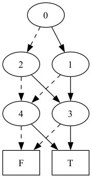
Importantly, the size of the BDD grows linearly with the length of the chain! This indicates that inference-via-compilation if achieving efficiency on this example (though, note that to achieve linear time, one must be careful about how one compiles and encodes.)
2.6 Search-based BDD compilation
Compositional BDD compilation is quite elegant, but it has some weaknesses. First, many intermediate BDDs are constructed along the way to the final BDD that may not end up being relevant. And second, the process of compiling the BDD may require repeatedly traversing intermediate BDDs, which can be expensive.
2.7 Circuit languages
Now we broaden our knowledge compilation map by considering more kinds of tractable languages, perhaps some that are more efficient to represent than BDDs, which may be too large. A natural avenue is to relax some structure of the BDD and see if that still yields a language with valuable properties. We will see that we can relax the variable order restriction, yielding new tractable languages that give up some structure (in particular, compositionality) in exchange for provably smaller representations.
A negation normal form (NNF) circuit is a directed acyclic graph consisting of (1) disjunction nodes \lor, (2) conjunction nodes \land, (3) leaves as literal. For example, the following is an NNF circuit:
NNFs include a broad class of circuit languages include CNF. Given a new language, it’s natural to ask what queries it can support efficiently. Unsurprisingly, NNF doesn’t give us much, since it’s so expressive: none of the queries we saw earlier are efficient for NNFs. In order to gain some queries, we need to add some structure:
These names are historical and were introduced in the original knowledge compilation map paper and prior work to it, but I think better names would be separation for decomposability and covering for determinism.
Definition (Decomposability): An and-node (\land) node in an NNF circuit is called decomposable if its two children do not share variables.
Definition (Determinism): An or node (\lor) node \varphi \lor \psi is deterministic if if its two children are mutually exclusive, i.e., \llbracket \varphi \land \psi \rrbracket = \llbracket F \rrbracket.
An NNF circuit that is decomposable is called DNNF, and an NNF circuit that is both decomposable and deterministic is called d-DNNF. As more structural properties are added, more efficient queries become possible.
2.7.1 A BDD is a d-DNNF Circuit
2.8 Compiling CNF to d-DNNF top-down
2.9 Beyond inference
Now we delve further into the benefits of knowledge compilation. So far, we’ve only performed efficient algorithms on the resulting compiled knowledge representation target, such as weighted model counting. But one of the amazing things about knowledge compilation is that they enable you to climb the complexity ladder: i.e., given a compiled representation, a query that used to be hard even given a counting oracle might suddenly become significantly more tractable. Adnan Darwiche calls this "climbing the complexity ladder."
Here is an example of a very useful query that is hard even with access to a counting oracle:
Definition (Marginal-MAP): Let \Pr(X, Y, Z) be a joint probability distribution on random variables X, Y, and Z. We call X the maximum a-posteriori (MAP) variables, Y the probabilistic variables, and Z the evidence. Then, the marginal-MAP query for evidence z is: \max_x \sum_y \Pr(X = x, Y = y \mid Z = z)
The marginal-MAP query is NP^{PP} hard, meaning it is NP-hard even with access to a counting oracle. Nonetheless, such queries are still solvable with knowledge compilation as long as we are strategic. Broadly there are two strategies: the first is to use variable-order constraints to place the MAP variables first in the order. The second is to use a branch-and-bound approach, first introduced by (Park and Darwiche 2004).
2.10 State of the art
Much of the knowledge compilation infrastructure we’ve seen in this lecture has been developed in tools, for example RSDD, a tool that my group works on. Knowledge compilers and knowledge compilation tools are quite mature and there are many existing open-source implementations:
BDD implementations.
d-DNNF compilers.
SDD compilers.
It is useful to mention here that there are approaches to evaluating queries besides knowledge compilation. For example, specialized probabilistic model counters like Ganak (Sharma et al. 2019) can scale better than knowledge compilers on certain problems for the specific task of model counting. There is a regular model counting competition that pushes the state of the art in model counting, see here.