1 Inference via Compilation
| #lang racket | package: base |
If we want probabilistic programming languages (PPLs) to be widely useful in practice as a tool for modeling and reasoning about uncertainty, they need to be fast and expressive. These two attributes are, of course, in tension: the more expressive the language is, the harder it is to make high-performance inference. Good language design strikes reasonable tradeoffs between these two attributes: we want as much expressivity as we can get without giving up too much performance.
This mini-course will be a deep dive into some of the algorithmic foundations for high-performance probabilistic inference. It will focus on knowledge compilation (Darwiche and Marquis 2002; Selman and Kautz 1996), an established foundation for high-performance exact probabilistic inference and other probabilistic reasoning tasks. Our central goal is to answer the question: how do we design algorithms that avoid the intractable worst-case hardness of probabilistic inference? This document is a literate programming document written in Racket; feel free to follow along with the code.
1.1 The Hardness of Inference
We begin by defining the foundational reasoning task for probabilistic programs: performing inference. We begin by defining a small probabilistic programming language called TinyPPL with the following surface syntax:
This is a discrete-valued probabilistic programming language without conditioning.
e ::= flip p |
| x <- e; e |
| pure e |
| if e then e else e |
| x |
| true |
| false |
TinyPPL is a standard monadic language with a pure and impure fragment that separates non-probabilistic from probabilistic computation. Now we can give a simple abstract syntax tree data structure in Racket that defines this language:
;; TinyPPL abstract syntax tree ;; monadic fragment: TinyPPLProb (struct Eflip (param) #:transparent) (struct Ebind (id assgn body) #:transparent) (struct Epure (p) #:transparent) ;; pure fragment: TinyPPLPure (struct Eite (g thn els) #:transparent) (struct Eid (id) #:transparent) (struct Etrue () #:transparent) (struct Efalse () #:transparent)
We can give TinyPPL a semantics in the standard style of (Reynolds 1972) by giving a definitional interpreter:
;; interp-pure : TinyPPLPure -> (Hashof Symbol Bool) -> Bool (define (interp-pure p env) (match p [(Etrue) #t] [(Efalse) #f] [(Eid x) (hash-ref env x)] [(Eite g thn els) (if (interp-pure g env) (interp-pure thn env) (interp-pure els env))])) ;; interp-prob : TinyPPLProb -> (Hashof Symbol Bool) -> Dist Bool (define (interp-prob e env) (match e [(Eflip p) (lambda (v) (if v p (- 1 p)))] [(Ebind x assgn body) (let* [(assgn-dist (interp-prob assgn env)) (body-t (interp-prob body (hash-set env x #t))) (body-f (interp-prob body (hash-set env x #f)))] (lambda (v) (+ (* (assgn-dist #t) (body-t v)) (* (assgn-dist #f) (body-f v)))))] [(Epure p) (let [(val (interp-pure p env))] (lambda (v) (if (equal? v val) 1 0)))]))
Now we can compute the semantics of small programs:
> (define p1 (Ebind 'x (Eflip 1/3) (Epure (Eid 'x)))) > (define dist1 (interp-prob p1 (hash))) > (dist1 #t) 1/3
As notation, we will use the semantic brackets \llbracket e \rrbracket to interpret programs according to the above semantics.
The problem of probabilistic inference is computing the semantics of a probabilistic program. To our dismay, the computational complexity of evaluating these semantics is very hard: indeed, it is as hard as counting the number of solutions to a Boolean formula. This class of problems is known as #P-hard problems.
Let’s see a quick reduction to establish this fact. Suppose we have a Boolean formula \varphi = (A \lor B) \land (\neg B \lor C). We want to count the number of models (solutions) to this formula by performing inference on a TinyPPL program. We can do it by running the following program:
Here we’ve made use of some simple syntactic sugar: one can easily desugar all logical operations like "and", "or", and "not" into an if-then-else.
A <- flip 1/2; |
B <- flip 1/2; |
C <- flip 1/2; |
pure (A or B) and (not B or C) |
If we perform inference on this program, we will get a probability that can be scaled up by 2^3 (the number of variables) to get the model count of \varphi.
This reduction is polynomial time: the resulting program is clearly polynomial in the size of \varphi. Hence, this reduction establishes that inference is at least as hard as model counting for Boolean formulae.
1.1.1 Why exact? Why discrete?
We have made two design choices in the above problem setup that you may be wondering about. First, we chose to focus on discrete-valued probabilistic programs: we only have facilities for making Bernoulli random variables. And second, we characterized only the hardness of exact probabilistic inference; what about approximations?
Discreteness is ubiquitous. Programs are naturally discrete: they have if expressions, they manipulate discrete data like graphs, etc. It is hard for one to avoid discrete random variables when using a probabilistic programming language, so we should be sure to handle them in our implementations.
Strategic problem simplification. Continuity is a powerful and expressive language feature, but it comes with a high burden: the semantics and inference implementations become vastly more complex when the state space is continuous. This makes it harder to implement algorithms, but it also makes it harder to analyze the worst-case complexity of those algorithms. So, we focus on exact inference for the sake of establishing foundations.
Exact inference is as hard as approximating (with guarantees). There is a classic (but, in my opinion, too-little-known) paper (Roth 1996) that establishes that approximations with guarantees are as hard as exact inference. This paper is highly recommended reading.
There is no substitute for the right answer. Approximate inference algorithms like rejection sampling, Hamiltonian Monte Carlo, etc. are great and they are widely-used. But, I will make a perhaps heretical claim: it’s not because we like them: it’s because they are what we have. The results from these inference algorithms are very hard to interpret and rely on because they are inherently stochastic. Many of the most widely-used approximations like Hamiltonian Monte Carlo have no correctness guarantees, because we do not know a-priori how long to run the Markov chain for. So, if we want PPLs to be used in high-consequence settings or in pedagagical settings, we need exact inference.
Exact inference can speed up approximate inference. We will return to this point in later lectures, but as foreshadowing, Rao-Blackwellization is a well-known and generic strategy for mixing exact and approximate inference.
Our goal is to work towards a scientific and systematic approach to probabilistic programming design. Hence, we strongly value things like guarantees on inference correctness and algorithmic analysis of inference performance.
1.2 When is inference efficient?
There are many valid notions of "size of program" we can use here. Let’s say, number of characters in the surface syntax representation.
Consider the following program, which we call a Markov chain of length 3:
x <- flip 1/2; |
x <- if x then flip 1/2 else flip 1/3; |
x <- if x then flip 1/2 else flip 1/3; |
pure x |
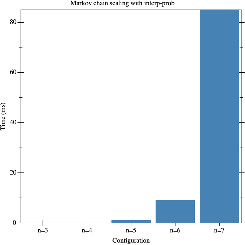
How does the cost of probabilistic inference scale in n? It is clear that our interp-prob function scales exponentially in n, since it scales exponentially in the number of flips in the program. We can observe this poor scalability quite easily by benchmarking a few example Markov chains:
The function make-chain is defined in tinyppl.rkt, and the bench function is defined in bench.rkt.
> (bench "Markov chain scaling with interp-prob" (list (list "n=3" (lambda () (interp-prob (make-chain 3) (hash)))) (list "n=4" (lambda () (interp-prob (make-chain 4) (hash)))) (list "n=5" (lambda () (interp-prob (make-chain 5) (hash)))) (list "n=6" (lambda () (interp-prob (make-chain 6) (hash)))) (list "n=7" (lambda () (interp-prob (make-chain 7) (hash))))))
1.2.1 Tractable Probabilistic Models
Inference is worst-case hard, but it is not always hard. Judea Pearl initiated the study of the algorithmic hardness of probabilistic inference in his seminal work on Bayesian belief networks (Pearl 2014).
In the Markov chain example above, we can see that the variable elimination algorithm efficiently performs inference. The core idea of variable elimination is to progressively simplify the program by marginalizing out (or eliminating) one variable at a time. For example, in the Markov chain above, we can eliminate the first assignment to x as follows:
x <- flip 5/12; |
x <- if x then flip 1/2 else flip 1/3; |
pure x |
The parameter to the first x is computed as \frac{1}{2} \times \frac{1}{2} + \frac{1}{2} \times \frac{1}{3}. We can continue eliminating the next assignment similarly:
x <- flip 29/72; |
pure x |
Crucially, each elimination step is local and efficient: each elimination step touches only the next line of code and always requires exactly 2 multiplications and an addition. Probabilistic models that admit efficient computation of inference are so essential that they get a special name:
Tractable probabilistic models are an active sub-area of research within the machine learning and artificial intelligence community today, and new ones continue to be developed.
Hence, a Markov chain is a tractable probabilistic, with the algorithmic witness to this fact being the variable elimination algorithm with topological elimination order. The observation that models with certain structure admit tractable inference was initially made by Pearl. Concretely, Pearl showed that for any polytree Bayesian network, the belief propagation algorithm converges to the correct distribution in time proportional to the diameter of the network. See (Pearl 2014) for more details.
1.3 Tractable Languages
"Computational efficiency is a central concern in the design of knowledge representation systems. In order to obtain efficient systems, it has been suggested that one should limit the form of the statements in the knowledge base or use an incomplete inference mechanism. The former approach is often too restrictive for practical applications, whereas the latter leads to uncertainty about exactly what can and cannot be inferred from the knowledge base. We present a third alternative, in which knowledge given in a general representation language is translated (compiled) into a tractable form—allowing for efficient subsequent query answering."
Bayesian networks and TinyPPL allows the programmer to write all sorts of models: some are tractable, some are intractable. It’s up to the programmer to write programs that run in a reasonable amount of time. These languages are (somewhat) expressive: they allow modelers to create many kinds of models, some of which scale, and some of which don’t. Now, we can put our language design hats on. Suppose we want to guarantee that all models written in a particular language are tractable. What do those tractable languages look like?
"[BDDs] are one of the only really fundamental data structures that came out in the last twenty-five years."
– Donald Knuth
In short, a BDD is a special kind of graphical representation of a Boolean formula. Let’s see a small example. Consider the Boolean formula:
(A \land B) \lor (\neg B \land C)
A binary decision diagram for this formula is:
> (define formula (Bor (Band (Bvar 0) (Bvar 1)) (Band (Bneg (Bvar 1)) (Bvar 2)))) > (define ex-bdd (formula->bdd formula)) > (render ex-bdd "bdd1")
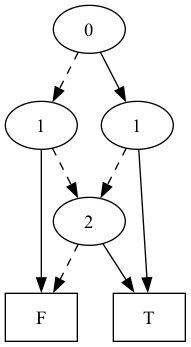
Let’s unpack this example BDD above and understand how to reaad it:
The BDD is a directed acyclic graph (DAG) and is read top-down.
Nodes are logical variables. We’ve numbered each of the logical variables: A is numbered 0, B is numbered 1, and C is numbered 2. The BDD is read top-down, and each node is labeled with a logical variable.
Leaves are truth values. At the bottom of the BDD is always T or F, denoting logical truthhood or falsehood.
Concretely, a BDD is an instance of a simple data structure:
> (struct BddNode (var high low) #:transparent)
The var field is the variable label, the high field is the solid edge, and the low field is the dashed edge. The BDD encodes the logical formula via its paths: each path from the root of the BDD to the T leaf encodes a model of the BDD. For example, the path 0=F, 1=T encodes the model A=T, B=F from the logical formula. A BDD is a compiled representation of a logical formula if and only if the models of the BDD are in one-to-one correspondence with the models of the formula.
Now that we know how to read a BDD, we can identify some of its more subtle inductive invariants give it important characteristics:
Variables are ordered from top to bottom of the BDD: 0 is first, then 1, then 2, etc. No variable can appear at more than a single level in the BDD.
BDDs are reduced. You may have noticed that there may be more than than 1 way to write a BDD corresponding to a single logical formula. For example, we could have two BDDs:
> (define b1 (BddNode 0 #t #t)) > (define b2 #t) The BDD b1 says "if 0 then #t else #t"; this is plainly the same as the BDD #t. In computer science we hate redundancy, so we want to eliminate this case: we say a BDD is reduced if no node has duplicate children. So, t1 is not reduced.
BDDs are canonical. For a fixed variable order, there is exactly 1 BDD representing any particular Boolean formula. It is easy to show (and a good exercise) that this canonicity property is a consequence of the ordering and reduced properties. It only makes sense to store only a single canonical version of every BDD in memory: this is why the variable 2 in the above example BDD has multiple incoming edges to it.
As we move through the course we will see how these special properties enable beautiful algorithms for manipulating and building BDDs, but for now, we will continue along with our high-level picture of what we can use BDDs for before returning to this topic.
1.3.1 Weighted model counting
And now we show how BDDs are tractable probabilistic languages by showing how they enable the efficient computation of probabilistic queries. But first we must answer the question: what is the probability distribution? So far, all BDDs can do is represent logical formulae.
There is a natural way to bring probabilities to the party: we can make each logical variable’s truth value an independent biased coin flip. Formally, we have the following setup:
The variable order for a BDD is a crucial parameter in ultimately determining the inference cost: different orders result in drastically different sized BDDs. We will return to this in the next lecture.
Suppose we have a finite set of logical variables X. Then, the sample space \Omega is the set of assignments to those logical variables, i.e. \Omega = X \rightarrow \{T,F\}. We write elements \omega \in \Omega as truth assignments like [A \mapsto T, B \mapsto F].
We give a probability measure \Pr : \Omega \rightarrow [0,1] that factorizes along logical variables: \Pr([X_1 \mapsto v_1, X_2 \mapsto v_2, \cdots, X_n \mapsto v_n]) = \Pr([X_1 \mapsto v_1]) \times \Pr([X_2 \mapsto v_2]) \times \cdots \times \Pr([X_n \mapsto v_n])
This is called a product distribution, since the distribution factorizes along the product structure of \Omega.
Now, we can associate Boolean formulae with random variables out of the above product distribution. Formally, given a Boolean formula \varphi, the reliability of \varphi is the probability that it evaluates to true under the above product distribution.
And now, the punchline: BDDs enable efficiently computing the reliability of a Boolean formula for any product distribution (Knuth 2009). The algorithm is a simple memoized recursive procedure:
(define (bdd-wmc f weightmap) (define/memo (bdd-wmc-h f) ; the define/memo macro creates a memoized procedure (match f [#t 1] [#f 0] [(BddNode v h l) (let [(sub-weight-h (bdd-wmc-h h)) (sub-weight-l (bdd-wmc-h l))] (+ (* (hash-ref weightmap v) sub-weight-h) (* (- 1 (hash-ref weightmap v)) sub-weight-l)))])) (bdd-wmc-h f))
The best way to understand this algorithm is to draw it on a BDD. It is a simple memoized procedure that works by computing the probability that the BDD evaluates to T. One can examine this algorithm to conclude that it runs in time linear in the size of the BDD: hence, BDDs are tractable languages.
In general this procedure is called weighted model counting. Given a Boolean formula \varphi and a weight map w that associates literals to real-valued weights, the weighted model count of \varphi is the weighted sum of models of \varphi, where the weight of each model is given as the product of the weights of each literal in that model:
\mathtt{WMC}(\varphi, w) = \sum_{m \models \varphi} \prod_{\ell \in m} w(\ell).
We will discuss this query – among other queries – in more detail next lecture. The pair (\varphi, w) is called a weighted Boolean formula.
1.4 Compiling to tractable languages
Now we can have a fresh perspective on the inference problem: inference can be a compilers problem. We can give the user a more expressive language like TinyPPL, a Bayesian network, or even a very expressive language like all of Scheme (Moy et al. 2025). Separately, we can explore and develop new tractable languages. And finally, we can bridge the gap between these two languages by compiling expressive high-level languages into low-level tractable languages. This pipeline is referred to as inference-via-compilation, and was introduced in the context of Bayesian inference by (Sang et al. 2005).
We will return to the topic of encoding probabilistic programs – and other probabilistic models – into Boolean formula in more detail in the third lecture.
ex ::= A <- flip 1/2; |
B <- flip 1/2; |
C <- flip 1/2; |
pure (A or B) and (not B or C) |
Here is a straightforward translation strategy: associate each flip with a logical variable whose weight is given by the parameter to the flip. Then, we can symbolically evaluate the program to extract a Boolean formula that encodes paths through the program. Concretely, the above program yields the following weighted Boolean formula and weight function:
\varphi = (f_A \lor f_B) \land (\neg f_A \lor f_C) w = [f_A \mapsto 1/2, \overline{f_A} \mapsto 1/2, f_B \mapsto 1/2, \overline{f_B} \mapsto 1/2, f_C \mapsto 1/2, \overline{f_C} \mapsto 1/2]
Notice we have that \llbracket \texttt{e} \rrbracket(T) = \mathtt{WMC}(\varphi, w): this relates computing semantics to a particular weighted model count. All that’s left to do is build a BDD for \varphi.
Conditional independence is not the only source of repetitious subfunctions in a logical formual, and hence conditional independence is not that only reason a BDD might be small for a particular probability distribution.
We have only discussed the size of the BDD but not the cost of building it. It might be expensive to build a BDD even if its ultimate size is small (a simple argument for this fact: suppose the final bdd is F; building this BDD might be as hard as SAT). We will discuss next lecture in more detail the cost of actually building the BDD, but the size of the BDD is a useful metric to keep in mind since it does closely correlate with cost.)
1.4.1 A growing trend of tractable compilation
There is a growing trend of inference-via-compilation in the probabilistic programming community, which I believe is due to the following factors:
Separation of concerns between language design and modeling. High-level language designers can focus on the challenge of designing semantics-preserving translations into target languages rather than the task of designing inference algorithms, similar to how LLVM frees language designers from the burden of understanding register allocation and optimization. Independently, designers of target languages can focus on the problem of designing efficient inference algorithms without concern for language usability, facilitating reuse of inference algorithms across language implementations.
Amortization of inference cost. In general the compilation step can be expensive, but once it is performed inference is guaranteed to be efficient in the size of the compiled representation. This provides several benefits. First, it enables new applications of PPLs to domains where guaran- teed runtime performance is paramount, for example real-time applications. Second, it enables tackling reasoning problems that go beyond inference, such as decision-making and optimization. These queries require repeated inference: the amortization of compilation facilitates development of new algorithms for solving these problems, which enables new features for high-level PPLs.
Avenues to a cost model. In general, it is very hard for programmers to know when inference algorithms will work well and when they won’t work well. Inference-via-compilation can provide programmers with a mental cost model of whether or not inference will be fast: for example, a programmer can visualize the BDD that a program might be compiled to, and use this to reason about its ultimate cost of performance.
Because of these benefits (and potentially others), inference-via-compilation is steadily becoming a standard tool in the probabilistic progamming language implementor’s toolbox. Let’s conclude with a brief historical tour through the development of inference-via-compilation up to its modern day application within the PPL community:
(Chavira and Darwiche 2008; Sang et al. 2005; Selman and Kautz 1996) Inference-via-compilation in Bayesian networks. These early works introduced the idea of inference-via-compilation in order to exploit context-specific independence (Boutilier et al. 2013). These early papers spurred on many of the developments in knowledge compilers, which we will explore in more detail next lecture.
Probabilistic logic programming. Inference-via-compilation made the jump to programming languages in 2011 in the context of the probabilistic logic programming language ProbLog (Fierens et al. 2011). ProbLog explored many of the early design choices that knowledge compilation enabled in the context of programming, including decision-making (Van den Broeck et al. 2010), semiring weighting (Kimmig et al. 2017), and machine learning (Manhaeve et al. 2018).
The next jump for knowledge compilation is into functional programming, initiated by my prior work (Holtzen et al. 2020). The key idea here is quite simple: the approach was to leverage symbolic execution to extract a Boolean formula from a program, in a manner identical to TinyPPL described in this lecture. Since then, many other projects have explored knowledge compilation in functional-style languages, including SPPL (Saad et al. 2021), Pluck (Bowers et al. 2025), noDice (Gürtler and Kaminski 2026), Roulette (Moy et al. 2025), and more (Garg et al. 2024; Li et al. 2023).
If I missed any compiled PPLs you know about, please let me know and I will add them!